TODO:
unique_fingerprint?I produced by emulator (emulate log(I)?)mo_gpDisclaimer: This code is an example only, and not (yet) a serious analysis. Results of the sensitivity analysis will change - perhaps dramatically - when sensible ranges for the parameters are used.
This code takes a small ensemble of runs of MetaWards runs and fits a Gaussian Process emulator to the maximum number of infections in each run. The code then does a sensitivty analysis using the FASTT99 algorithm, and emulated output. Finally, it looks at the one-at-a-time sensitivity using emulated output.
library(tidyverse)
library(sensitivity)
## Registered S3 method overwritten by 'sensitivity':
##   method    from
##   print.src dplyr
##
## Attaching package: 'sensitivity'
## The following object is masked from 'package:dplyr':
##
##     src
library(DiceKriging)
source("https://raw.githubusercontent.com/dougmcneall/packages-git/master/emtools.R")
Load the design file created in metawards_design.md:
# Need to fix the parameter names
design_file = 'https://raw.githubusercontent.com/dougmcneall/covid/master/experiments/2020-05-07-sensitivity-analysis/design.csv'
X <- read.csv(design_file, sep = "")
parnames = colnames(X)
Load the output file created in metawards_design.md. The output file used here can be downloaded from https://github.com/dougmcneall/covid/blob/master/experiments/2020-05-07-sensitivity-analysis/output/results.csv.bz2
# A container for all the data
# Each row has a "fingerprint" that contains the
# values of all the changed parameters, and the values of the parameters are also
# given.  This alters the order of the parameters.
dat <- read.csv('results.csv.bz2')
unique_fingerprint = unique(dat$fingerprint)

# find maximum number of infections for each ensemble member
max_infections <- dat %>%
                  group_by(fingerprint) %>%
                  summarize(max(I))

reorder_ix <- match(unique_fingerprint, max_infections$fingerprint)
max_infections <- max_infections[reorder_ix, ]

head(max_infections)
## # A tibble: 6 x 2
##   fingerprint                                                           `max(I)`
##   <chr>                                                                    <int>
## 1 0_0396911522:0_5487738012:0_4820402197:0_4917127313:0_7742976767:0_6…    14011
## 2 0_7294788517:0_4236460749:0_5140176034:0_7666981902:0_4031789148:0_4… 10625619
## 3 0_2940997886:0_7397552424:0_5851974157:0_5933214784:0_6098004712:0_4…  5952759
## 4 0_4117703374:0_5074890216:0_3288689441:0_4084163311:0_8264602178:0_4…  1853024
## 5 0_5366404451:0_7915200822:0_7097633424:0_7255256459:0_4756592319:0_3… 11130717
## 6 0_6555091723:0_348384008:0_5585651195:0_4524178774:0_3879190864:0_13… 20328204
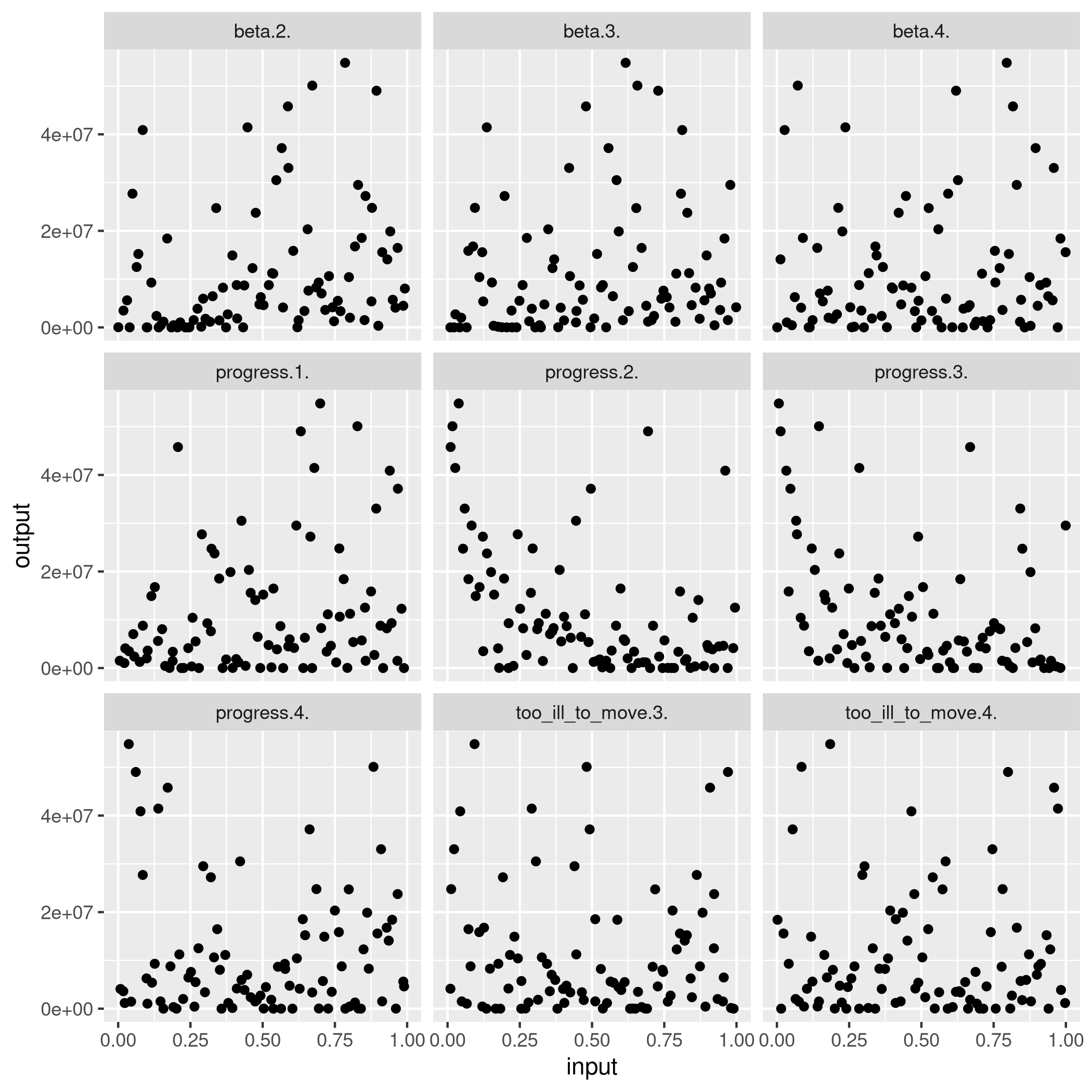
Plot each parameter against the output to get an idea of sensitivity
d <- ncol(X)
X.norm <- normalize(X)
y <- pull(max_infections,'max(I)')
X %>%
  as_tibble %>%
  mutate(y=y) %>%
  gather('parameter', 'value', -y) %>%
  ggplot(aes(x=value, y=y)) +
    geom_point() +
    facet_wrap(~parameter) +
    labs(y='output', x='input')
# Fit an emulator using DiceKriging
fit = km(~., design=X.norm, response=y)
##
## optimisation start
## ------------------
## * estimation method   : MLE
## * optimisation method : BFGS
## * analytical gradient : used
## * trend model : ~beta.2. + beta.3. + beta.4. + progress.1. + progress.2. + progress.3. +
##     progress.4. + too_ill_to_move.3. + too_ill_to_move.4.
## * covariance model :
##   - type :  matern5_2
##   - nugget : NO
##   - parameters lower bounds :  1e-10 1e-10 1e-10 1e-10 1e-10 1e-10 1e-10 1e-10 1e-10
##   - parameters upper bounds :  2 2 2 2 2 2 2 2 2
##   - best initial criterion value(s) :  -1550.089
##
## N = 9, M = 5 machine precision = 2.22045e-16
## At X0, 0 variables are exactly at the bounds
## At iterate     0  f=       1550.1  |proj g|=       1.8294
## At iterate     1  f =       1536.9  |proj g|=        1.4146
## At iterate     2  f =       1532.1  |proj g|=        1.9459
## At iterate     3  f =       1526.3  |proj g|=        1.9138
## At iterate     4  f =       1524.9  |proj g|=        1.8521
## At iterate     5  f =       1523.1  |proj g|=        1.7403
## At iterate     6  f =       1521.3  |proj g|=        1.6157
## At iterate     7  f =       1520.9  |proj g|=        1.5526
## At iterate     8  f =       1520.3  |proj g|=        1.0518
## At iterate     9  f =       1520.1  |proj g|=       0.53761
## At iterate    10  f =       1519.6  |proj g|=        1.5438
## At iterate    11  f =       1519.5  |proj g|=       0.83068
## At iterate    12  f =       1519.5  |proj g|=       0.75584
## At iterate    13  f =       1519.5  |proj g|=       0.48607
## At iterate    14  f =       1519.5  |proj g|=       0.10189
## At iterate    15  f =       1519.4  |proj g|=      0.028111
## At iterate    16  f =       1519.4  |proj g|=      0.049962
## At iterate    17  f =       1519.4  |proj g|=       0.10369
## At iterate    18  f =       1519.4  |proj g|=        0.1459
## At iterate    19  f =       1519.4  |proj g|=      0.036488
## At iterate    20  f =       1519.4  |proj g|=     0.0073222
## At iterate    21  f =       1519.4  |proj g|=     0.0018967
##
## iterations 21
## function evaluations 23
## segments explored during Cauchy searches 29
## BFGS updates skipped 0
## active bounds at final generalized Cauchy point 4
## norm of the final projected gradient 0.00189674
## final function value 1519.45
##
## F = 1519.45
## final  value 1519.449375
## converged
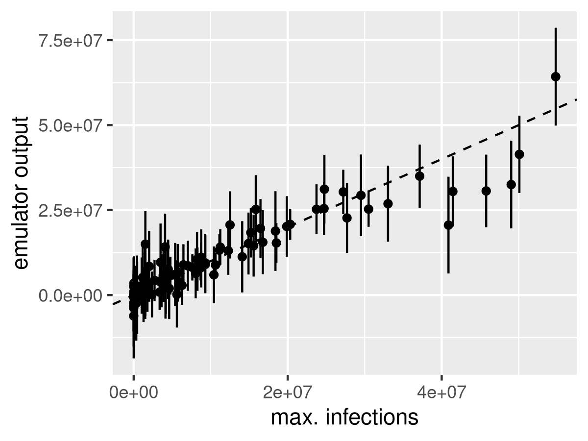
loo = leaveOneOut.km(fit, type = 'UK', trend.reestim = TRUE)

tibble(y=y, em_mean=loo$mean, em_sd = loo$sd) %>%
  ggplot() +
  geom_segment(aes(x=y, xend=y, y=em_mean - 2*em_sd, yend=em_mean + 2*em_sd)) +
  geom_point(aes(x=y, y=em_mean)) +
  geom_abline(intercept=-1, slope=1, lty=2) +
  labs(x='max. infections', y='emulator output')
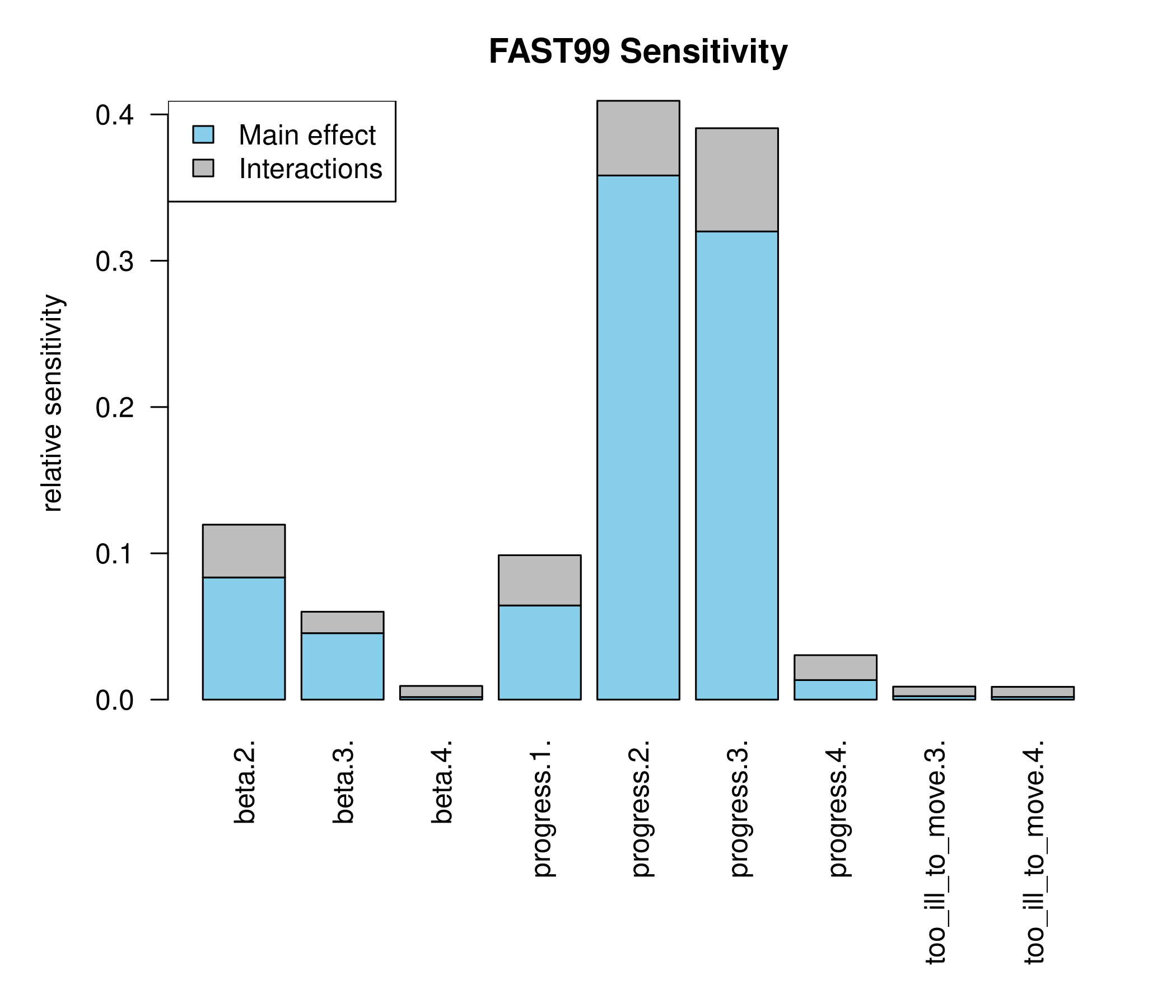
cf. Saltelli et al (1999)
# Generate a design for the FAST99 analysis
X.fast <- fast99(model = NULL, factors = colnames(X), n = 3000,
                 q = "qunif", q.arg = list(min = 0, max = 1))


# Predict the response at the FAST99 design points using the emulator
pred.fast = predict(fit, newdata = X.fast$X, type = 'UK')

# Calculate the sensitivity indices
fast.tell <- tell(X.fast, pred.fast$mean)

bp.convert <- function(fastmodel){
  # get the FAST summary into an easier format for barplot
  fast.summ <- print(fastmodel)
  fast.diff <- fast.summ[ ,2] - fast.summ[ ,1]
  fast.bp <- t(cbind(fast.summ[ ,1], fast.diff))
  fast.bp
}
par(las = 2, mar = c(9,5,3,2))
barplot(bp.convert(fast.tell), col = c('skyblue', 'grey'),
        ylab = 'relative sensitivity',
	main = 'FAST99 Sensitivity')
##
## Call:
## fast99(model = NULL, factors = colnames(X), n = 3000, q = "qunif",     q.arg = list(min = 0, max = 1))
##
## Model runs: 27000
##
## Estimations of the indices:
##                    first order total order
## beta.2.            0.083486681 0.119576749
## beta.3.            0.045428226 0.060061735
## beta.4.            0.001766290 0.009332883
## progress.1.        0.064347083 0.098696670
## progress.2.        0.358255653 0.409314287
## progress.3.        0.320019815 0.390562790
## progress.4.        0.013345921 0.030384966
## too_ill_to_move.3. 0.002378786 0.008862051
## too_ill_to_move.4. 0.001826869 0.008733377
legend('topleft',legend = c('Main effect', 'Interactions'),
       fill = c('skyblue', 'grey') )
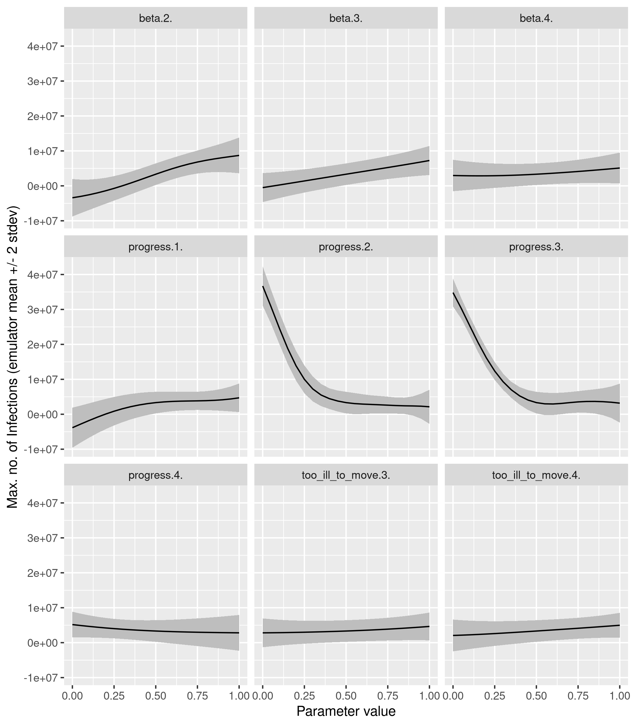
Parameters are swept across their range one at a time, with the remaining parameters held at central values.
n.oat <- 21
X.oat <- oaat.design(X.norm, n = n.oat, hold = rep(0.5,9))

colnames(X.oat) <- colnames(X)
pred.oat <- predict(fit, newdata = X.oat, type = 'UK')
params = rep(colnames(X.oat), each=n.oat)
col_inds = rep(1:ncol(X.oat), each=n.oat)
tibble(parameter = params,
       value = X.oat[cbind(1:length(col_inds), col_inds)]) %>%
  mutate(pred_mean=pred.oat$mean,
	 pred_sd=pred.oat$sd,
	 lwr = pred_mean - 2 * pred_sd,
	 upr = pred_mean + 2 * pred_sd) %>%
  ggplot(aes(x=value)) +
    geom_ribbon(aes(ymin=lwr, ymax=upr), fill='gray') +
    geom_line(aes(y=pred_mean)) +
    facet_wrap(~parameter) +
    labs(x='Parameter value', y='Max. no. of Infections (emulator mean +/- 2 stdev)')