UQ4Covid

library(sf)
library(tidyverse)
library(leaflet)
library(htmltools)

Goal

This is a walk-through tutorial to get from MetaWards output to a map plot (choropleth). The code presented here can be used to write custom functions for easy plotting of model output.

Wards boundaries

Note: This section is only for completeness, to run the code simply jump to the next section.

The 2011 census ward boundaries shapefile were be downloaded from statistics.digitalresources.jisc.ac.uk. I used the mapshaper command line tool (see https://github.com/mbloch/mapshaper) to reduce the number of points and thus bring the filesize down from 350Mb to about 3Mb. The mapshaper shell commands used were

mapshaper infuse_ward_lyr_2011.shp -simplify visvalingam 0.005 \
          -o force infuse_ward_lyr_2011_coarse.shp
mapshaper infuse_ward_lyr_2011_coarse.shp snap snap-interval=100 \
          -o force infuse_ward_lyr_2011_coarse.shp

Then I transformed the spatial polygons data frame to a sf object in the proper projection and saved it for later use:

library(rgdal)
wards_sf = readOGR('infuse_ward_lyr_2011', 'infuse_ward_lyr_2011_coarse') %>%
           st_as_sf() %>%
           st_cast('MULTIPOLYGON') %>%
           st_transform('+proj=longlat +datum=WGS84 +no_defs') %>%
	   rename(WD11CD = geo_code)
save(file='wards_sf.Rdata', list='wards_sf')

Load wards data

load('wards_sf.Rdata')

An interactive map of the raw wards boundary data can be displayed in the browser with

# not run:
leaflet(wards_sf) %>% 
  addTiles() %>% 
  addPolygons(col='black', weight=1)

Import Metawards output and calculate maximum number of infections per ward

Next we load a MetaWards model output. Here we use the file wards_trajectory_I.csv.bz2 from the 0i3v0i0x001 run in the experiment here.

The outputs in this experiment are timeseries of number of infections for each ward. We extract only the day and ward* columns and calculate the maximum number of infections per ward:

# load metawards output 
mw_output = read.csv('wards_trajectory_I.csv.bz2')

# transform to tbl and calculate max. number of infections per ward
max_infect = 
  mw_output %>% 
  as_tibble %>%
  select(day, starts_with('ward')) %>%
  gather('ward', 'infect', -day) %>%
  group_by(ward) %>%
  summarise(max_infect = max(infect))

Next we remove ward[0] and extract the integer index of each ward so we can later match them with the ward ID from the MetaWards lookup table.

# remove ward 0, extract ward index from col name, and match with ward id
max_infect_ward =
  max_infect %>%
  filter(ward != 'ward.0.') %>%
  mutate(FID = as.numeric(str_extract(ward, '\\d+')))

Import ward lookup table

The MetaWards ward lookup table Ward_Lookup.csv was downloaded from here. The first column holds the ward id (WD11CD) which we extract and join it with maximum infections data frame on column name FID. The WD11CD is also a column in the wards boundaries data so it will be used to combine the data frames later.

metawards_lookup = read.csv('Ward_Lookup.csv') %>%
	as_tibble %>%
	select(WD11CD, FID)
max_infect_ward = left_join(max_infect_ward, metawards_lookup, by='FID')

NOTE: not all MetaWards wards are in the boundaries data set

setdiff(metawards_lookup$WD11CD, wards_sf$WD11CD)

##  [1] "E05003230" "E05003216" "W05000053" "W05000055" "W05000058" "W05000068"
##  [7] "W05000080" "W05000081" "W05000082" "W05000083" "W05000084" "W05000088"
## [13] "W05000294" "W05000300" "W05000309" "W05000001" "W05000108" "W05000035"
## [19] "W05000041" "W05000045" "W05000047" "W05000050" "W05000320" "W05000604"
## [25] "W05000954" "W05000958" "W05000896" "E05006972" "E05006554" "E05006566"
## [31] "E05000002" "E05000003" "E05000004" "E05000005" "E05000006" "E05000007"
## [37] "E05000008" "E05000009" "E05000010" "E05000011" "E05000012" "E05000013"
## [43] "E05000014" "E05000016" "E05000017" "E05000018" "E05000019" "E05000020"
## [49] "E05000021" "E05000022" "E05000023" "E05000024" "E05000025" "E05006982"
## [55] "E05008322" "E05008323" "E05008324" "E05008325" "E05008326" "E05005228"
## [61] "E05005246"

Join MetaWards and boundary data sets

Now matching infection data from the model run to the ward boundaries is a simple merge by WD11CD:

# merge data frames
max_infect_df = merge(wards_sf, max_infect_ward, by='WD11CD')

Static plot

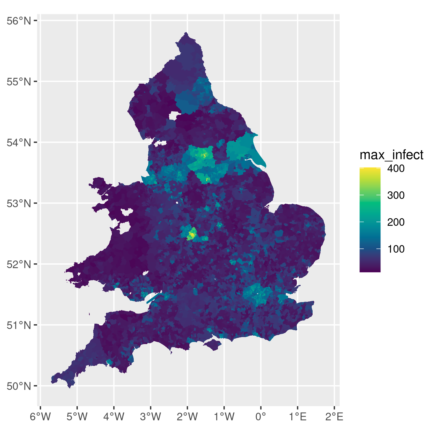
# ggplot object (13Mb)
plt = ggplot(max_infect_df) + 
        geom_sf(aes(fill=max_infect), lwd=0) + 
        scale_fill_gradientn(colours=hcl.colors(n=10))

# show
plt

# to save:
# ggsave('plot.png', plt)

Interactive plot

# not run:
palette = colorNumeric(palette="viridis", domain=max_infect_df$max_infect)

max_infect_df = max_infect_df %>%
  mutate(text = paste(name, max_infect, sep=': '))

map = leaflet(max_infect_df) %>% 
        addTiles() %>% 
        addPolygons(fillColor=~palette(max_infect), fillOpacity=0.9, 
                    col='black', weight=2, label = ~htmlEscape(text)) %>% 
        addLegend(pal=palette, values=~max_infect, opacity=1, 
                  title='Maximum no\n of infections')

# to show map in browser do
# print(map)

# save as html widget
htmlwidgets::saveWidget(map, file='metawards_output_map.html')

Load libraries